Temporal Uncertainty
Temporal is related to time, which is a (quantitative) continuous variable, while uncertainty refers to situations involving unknown information.
(see also Time and dating)
Monte-Carlo simulation tests the significance of the observed fluctuations in the context of uncertainty in the calibration curve and [archaeological] sampling.
Probability and uncertainty
We can apply a probabilistic approach when dealing with uncertainty. In this case, uncertainty is considered a measure quantifying the likelihood that events will occur.
Different approaches for assigning probabilities include:
the proportion of a particular outcome to all possible outcomes (classical)
the long-run relative frequency of the probability for an outcome to occur
certain degree of belief (subjective)
Probability space
A probability space defines an occurrence or event as a subset of that space.
For example, if the probability space is the interval \([0,1]\), with the uniform distribution then the interval \([ \frac{1}{3}, 1 ]\) is an event that represents a randomly chosen number between \(0\) and \(1\) turning out to be at least \(\frac{1}{3}\).
Probability distributions
A probability distribution describes the associated probability of possible outcomes for a random variable \(X\).
For a single variable, the data is allocated in univariate distributions, and we use multivariate distributions to infer on multiple parameters.
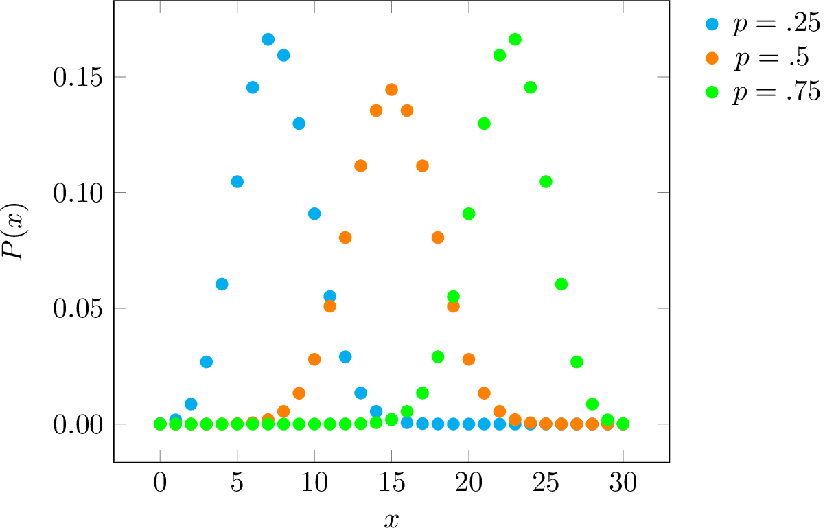
Binomial distribution
A binomial distribution is a continuous distribution that describes a binomial experiment where there are two possible outcomes.
The probability mass function (p.m.f.) corresponding to the binomial distribution represents the probability of \(x\) successes in a binomial experiment
\(P(x) \;=\; {n\choose x} ~p^x (1-p)^{n-x}\)
where \(P(x)\) is the distribution function for the probability of success for \(x = 0, 1, 2, \dots, n\).
|
A plot of the binomial distribution for \(n=30\) and with different \(p\) values.
Note
The Bernoulli distribution is a special case of the binomial distribution when \(n = 1\).
Note
The Beta distribution models the probability \((p)\) of success rather than the number of occurrences \((x)\), and it represents all the possible values of \((p)\) when we do not know what that probability is.
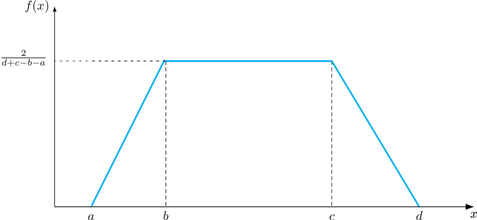
Trapezoidal distribution
Trapezoidal distributions seems appropriate for modeling the duration and the form of a phenomenon with a growth-stage, relative stability, and decline. These three parameters are not necessarily similar and an occurrence can have, for example, a long development and abrupt decay.
The probability density function of the trapezoidal distribution for \(a \leqslant b \leqslant c \leqslant d\) is
\(f(x \mid a,b,c,d) = \begin{cases}U \bigl(\frac{x-a}{b-a}\bigr) \quad a \leqslant x < b\\U \qquad b \leqslant x < c\\U \bigl(\frac{d-x}{d-c}\bigr) \quad c \leqslant x < d\\ 0 \quad \text{elsewhere}\end{cases}\)
where \(U = 2(d + c - b - a)^{-1}\) corresponds to the uniform distribution.
|
A trapezoidal distribution where decline is longer than growth.
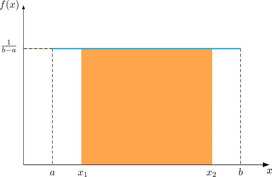
Uniform distribution
The uniform distribution is a special case of a trapezoidal distribution with a constant probability.
The probability density function of the continuous uniform distribution for \(a \leqslant x \leqslant b\)
\(f(x) \;=\; \frac{1}{b-a}\)
and \(f(x) = 0\) iff \(x<a\) or \(x>b\)
|
Uniform distribution plot for \(P(x_1 < X < x_2)\).
Note
There is also a discrete version of the uniform distribution that is a generalization of the Bernoulli distribution.
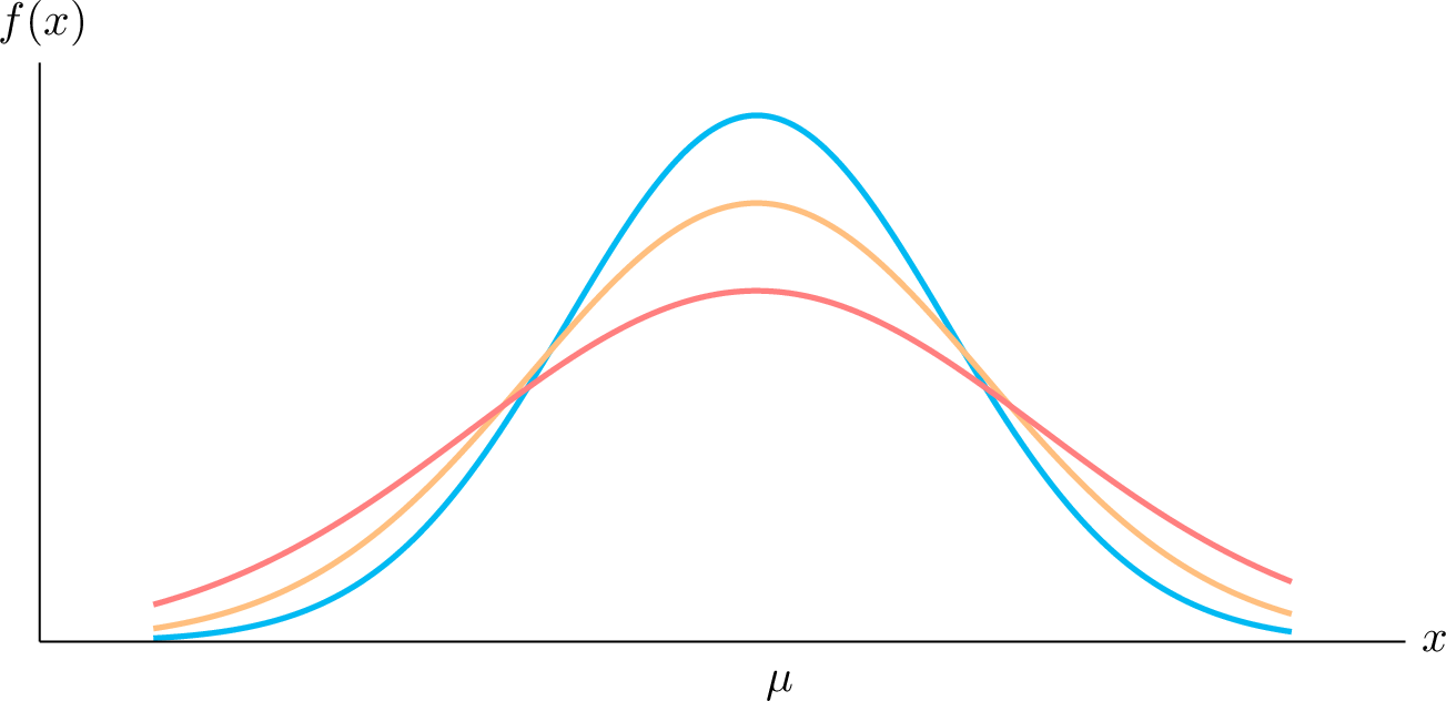
Normal distribution
The normal distribution –or “bell curve”– is the probability distribution for a normal random variable \(X \sim N (\mu,\sigma^2)\). The normal distribution is also called Gaussian distribution due to C.F. Gauss who described this distribution in mathematical terms.
The normal distribution is the most important distribution in statistics, and play a crucial role in statistical inference. This is partly because it approximates well the distributions of many types of variables.
The exact form of the distribution depends on the values of the mean \(\mu\) and the standard deviation \(\sigma\) parameters.
The probability density function of a normal random variable \(-\infty < x < \infty\) is:
\(f(x) \;=\; \frac{1}{{\sigma \sqrt {2\pi } }}\;e^{{{ - \frac12 \left( \frac{x - \mu }{\sigma} \right)^2 } }}\)
where \(e \approx 2.7183\) (Euler’s number), and \(\pi \approx 3.1416\) (Pi number).
Note
A special case of the normal distribution with mean \(\mu = 0\) and standard deviation \(\sigma = 1\) is the standard normal distribution \(Z\). Any arbitrary normal distribution can be converted to \(Z\).
|
Normal distributions with different variances \(\sigma^2\) and same mean \(\mu\).
Todo
Expectations of the distributions.
Notation
To study temporal uncertainty, the following notation is adopted:
\(\varOmega =\) range of time
\(\tau =\) time span of existence
\(\Delta \tau =\) duration of \(\tau\)
\(t_i =\) a given portion of time
\(\Delta t_i =\) duration of \(t_i\)
\(\varphi =\) temporal resolution
\(e =\) event or occurrence
\(P, p =\) probability
Aoristic analysis
Aoristic analysis is based on the creation of a series of these artificial divisions of the range of time with a fixed value, called time blocks, and the definition of their probability of existence.
Boundaries of existence
Limits of dating for events are the earliest and the latest time the event may have happened. These upper and lower bounds are termed
terminus ante quem (TAQ) or “limit before which”
terminus post quem (TPQ) or “limit after which”
Temporal resolution
Temporal resolution \(\varphi\) refers to the duration of time blocks, and with aoristic analysis \(\varphi\) is fixed.
Aoristic sum
A proxy for evaluating change in the total counts of events across time is the aoristic sum, which is the sum of probabilities for each time block.
The aoristic sum is computed accross the sum of probabilities for events in a single portion of time \(t_i\).
    t1  t2  t3
     ^   ^   ^
a    |   |   |
b    |   |   |
c    |   |   |
     ^   ^   ^
     aoristic
       sums
Todo
Aoristic sum explained in R…
Probability of existence \(t_i\)
The probability of existence \(p[t_i]\) of an event \(e\) in a range of time \(\varOmega\) is the probabilty distribution
\(p[t_i] = \Delta t_i / \Delta \tau\)
where \(\tau\) is the time span of existence, \(\Delta\) is for the duration of a given portion of time \(t_i\) or of \(\tau\).
To compute \(p[t_i]\), Crema (2012, p. 447) takes the following example (years are BC):
350 ---- 300 ---- 250
     t1       t2

     342 ---- 288
         tau
Hence, \(\Delta \tau\) in this case is \(54\).
Time-block boundaries
To retrieve the minimum probability \(P[\varphi_\alpha]\) for the boundaries of the first and last time-blocks, we define \(\varphi_\alpha = 1\) where
\(\phi_\alpha / \Delta_\tau = 1/54 = P[\phi_\alpha] = .018\) (approx)
Hence, the probability of existence for \(t_1\)
\(P[t_1] = P[\phi_\alpha] \cdot 42\)
(i.e. \(342 - 300\))
\(P[t_1] = .018 \cdot 42 = .78\)
The probability of existence for for \(t_2\)
\(P[t_2] = P[\phi_\alpha] \cdot 12\)
(i.e. \(300 - 288\))
\(P[t_2] = .018 \cdot 12 = .22\)
Etc.
Assumption (among others): Any equally long portion of time within the time span \(\tau\) has the same probability of existence.
Probabilities of existence for time blocks
The probability of existence for each time block (Appendix A, Crema, 2012)
\(P_b \;=\; {\sum_{i=0}^{\pi-1} \sum_{j=1}^{d/\varphi} \theta (i+j,\;b)} / {\pi}\)
where \(\pi\) is the number of all possible permutations, and \(b\) is a numerical index of temporal blocks within \(\tau\).
On the other hand, the number of all possible permutations \(\pi\) equals \({(\Delta \tau - d)}/{\varphi + 1}\) where \(d\) is the duration of \(e\).
Note
\(d\) is rounded to the value of the temporal resolution, and \(b\) ranges from \(1\) to \(\Delta t_i/\varphi\), which are the edges of the time span.
Temporal resolution for time blocks
The duration of time blocks that is \(\varphi\) in the denominator for computing \(\pi\) is known as the temporal resolution, while the numerator expression for the probability of existence for each time block is defined as
\(\theta (i+j,\;b) = \begin{cases}1 \quad \text{if}\; i+j = b \\ 0 \quad \text{if}\; i+j \neq b \end{cases}\)
Rate of change
Rate of change refers to transition probabilities like increase/stability/decrease as with the trapezoidal distribution.
Rate of chage = \(\frac{(e~t_{i+1} - e~t_i)}{\varphi}\)
An example of a transition probabilities are increase \(=0.4\); stability \(=0.5\) and decrease \(=0.1\)
Computing the probability of existence
We use function prex() to compute the probability of existence.
-
prex()
Function usage
# probability of existence
R> prex(x, taq, tpq, vars, bins = NULL, cp, aoristic = TRUE, weight = 1,
        DF, out, plot = FALSE, main = NULL, ...)
Parameters
x:
list or data frame object of variables and observations.
taq:
TAQ or terminus ante quem
tpq:
TPQ or terminus post quem
vars:
boundaries of existence in
x(vector for TAQ and TPQ)bins:
length of the break (integer)
cp:
chronological phase (optional)
aoristic:
return aoristic sum? (logical)
weight:
weight to observations
DF:
return also data frame with observations? Ignored for plot (logical and optional)
out:
number of outliers to omit (integer or vector where first entry id for latest date)
plot:
plot the results? (logical and optional)
main:
plot’s main title (optional)
…:
additional optional parameters
Details
In case that bins is NULL, then the time breaks take the chronological period specified in cp, which by
default is "bin5" or a five-periods model for the EDH dataset; the other built-in option is "bin8" for eight
chronological periods. Argument cp is open for other chronological phases as long as they are recorded as a list object.
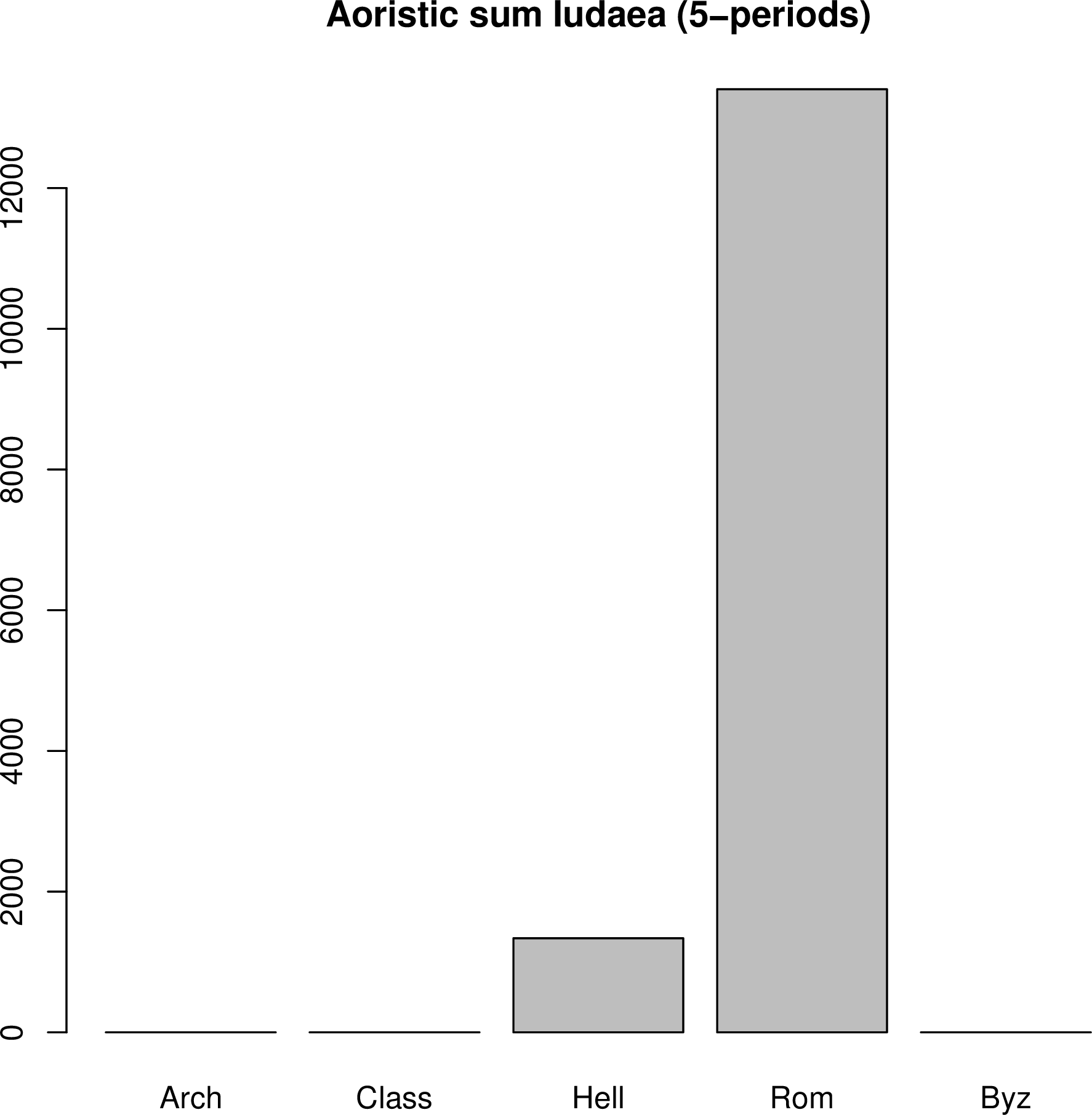
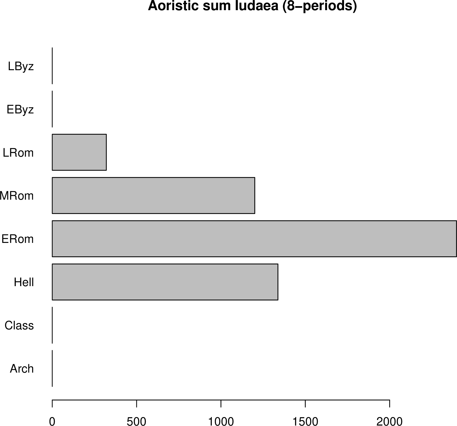
For example, the (default) aoristic sum of EDH inscriptions in the Roman province
of Iudaea computed with prex()
# get inscriptions from Iudaea in EDH data base
R> iud <- get.edh(search="inscriptions", province="Iud")

# 5-chronological periods
R> prex(x=iud, taq="not_before", tpq="not_after", cp="bin5")
#  Arch     Class      Hell       Rom       Byz
# 0.000     0.000  1337.904 13405.017     0.000

# 8-chronological periods
R> prex(x=iud, taq="not_before", tpq="not_after", cp="bin8")
#  Arch     Class      Hell      ERom      MRom      LRom      EByz      LByz
#0.0000    0.0000 1337.9040 2396.4529 1200.5623  320.5379    0.0000    0.0000
Plotting aoristic sum
To visualize the aoristic sum from the Roman province of Iudaea or iud as bar plots with function prex()
and two types of chronological phases
#  five chronological phases
R> barplot(prex(x=iud, taq="not_before", tpq="not_after", cp="bin5"),
+          main="Aoristic sum Iudaea (5-periods)" )

# eight chronological phases
R> barplot(prex(x=iud, taq="not_before", tpq="not_after", cp="bin8"),
+          horiz=TRUE, las=1, main="Aoristic sum Iudaea (8-periods)" )
that produce
|
|