Time and dating
Time is a (quantitative) continuous variable, but we often think time as a discrete variable since is rounded when measured (e.g. a person is 40 years old and not between 40 and 41).
Chronological periods of the Mediterranean Sea
We use chronological periods for dating purposes. Sometimes chronological periods are divided by phases and occasionally they are referred as chronological phases.
For example, chronological phases for dating ancient cultures of the Mediterranean Sea are
Chronological phase |
Absolute dates (approx.) |
|---|---|
Middle to Late Neolithic (MN-LN) |
6000-4500 BC |
Final Neolithic to Early Bronze 1 (FN-EB1) |
4500-2700 BC |
Early Bronze 2 (EB2) |
2700-2200 BC |
Late Prepalatial (LPrepal) |
2200-1900 BC |
First Palace (FPal) |
1900-1700 BC |
Second Palace (SPal) |
1700-1450 BC |
Third Palace (TPal) |
1450-1200 BC |
Post-Palatial to Protogeometric (PPalPg) |
1200-900 BC |
Geometric (Geo) |
900-700 BC |
Archaic (Arch) |
700-500 BC |
Classical (Class) |
500-325 BC |
Hellenistic (Hell) |
325 BC - AC 0 |
Early Roman (ERom) |
AC 0-200 |
Middle Roman (MRom) |
AC 200-350 |
Late Roman (LRom) |
AC 350-650 |
Early Byzantine (EByz) |
AC 650-900 |
Middle Byzantine (MByz) |
AC 900-1200 |
Early Venetian (EVen) |
AC 1200-1400 |
Middle Venetian (MVen) |
AC 1400-1600 |
Late Venetian (LVen) |
AC 1600-1800 |
Recent (Recent) |
AC 1800-present |
(adapted from Bevan et al, 2013 (doi: 10.1111/j.1475-4754.2012.00674.x))
AC is sometimes ommited, and a negative number represents BC.
Relative dating of Roman inscriptions
Since the range of time in the relative dating of Roman inscriptions without outliers is between 530 BC and 950 AC, the chronological periods involving epigraphic Roman material are
Period |
Dates years |
|---|---|
Archaic (Arch) |
-700 to -500 |
Classical (Class) |
-500 to -325 |
Hellenistic (Hell) |
-325 to 0 |
Early Roman (ERom) |
0 to 200 |
Middle Roman (MRom) |
200 to 350 |
Late Roman (LRom) |
350 to 650 |
Early Byzantine (EByz) |
650 to 900 |
Middle Byzantine (MByz) |
900 to 1200 |
The eight chronological phases are reduced to five categories with their respective years:
Period |
Dates years |
|---|---|
Archaic (Arch) |
-700 to -500 |
Classical (Class) |
-500 to -325 |
Hellenistic (Hell) |
-325 to 0 |
Roman (Rom) |
0 to 650 |
Byzantine (Byz) |
650 to 1200 |
Eight- and five chronological phases are for the analysis of temporal uncertainty of the EDH dataset.
Dates in data frames
To produce data frames, we need to make explicit with the as argument; in the
example below with chronological data in the function where "id" is added by default.
# produce a data frame with chronological data variables and remove missing data
R> EDHdates <- edhw(vars=c("not_after", "not_before"), as="df")
The first entries are
# look at the first ones
R> head(EDHdates)
#        id not_before not_after
#1 HD000001       0071      0130
#2 HD000002       0051      0200
#3 HD000003       0131      0170
#4 HD000004       0151      0200
#5 HD000005       0001      0200
#6 HD000006       0071      0150
and the last entries
# look at the last ones
R> tail(EDHdates)
#            id not_before not_after
#83816 HD081504       0071      0130
#83817 HD081505       0071      0130
#83818 HD081506       0071      0130
#83819 HD081507       0101      0200
#83820 HD081508       0151      0230
#83821 HD081509       0151      0250
Time spans of existence
Object EDHdates has information about relative dating with boundaries of existence
in variables not_before and not_after.
In EDHdates, however, these variables are factors and they need to be converted into vectors
with a numeric format in order to represent the boundaries of existence.
# time columns in EDHdates are factors
R> is.factor(EDHdates$not_after)
R> is.factor(EDHdates$not_before)
#[1] TRUE

# boundaries of existence not_before and not_after
R> nb <- as.numeric(as.vector(EDHdates$not_before))
R> na <- as.numeric(as.vector(EDHdates$not_after))
To compute oldest and latest years with min and max functions, we also need to remove NA
data from these vectors.
# oldest and latest dates
R> years <- c(min(nb, na.rm=TRUE), max(na, na.rm=TRUE))
#[1] -530 1998
Dates in years are between 530 BC and 1998 AC.
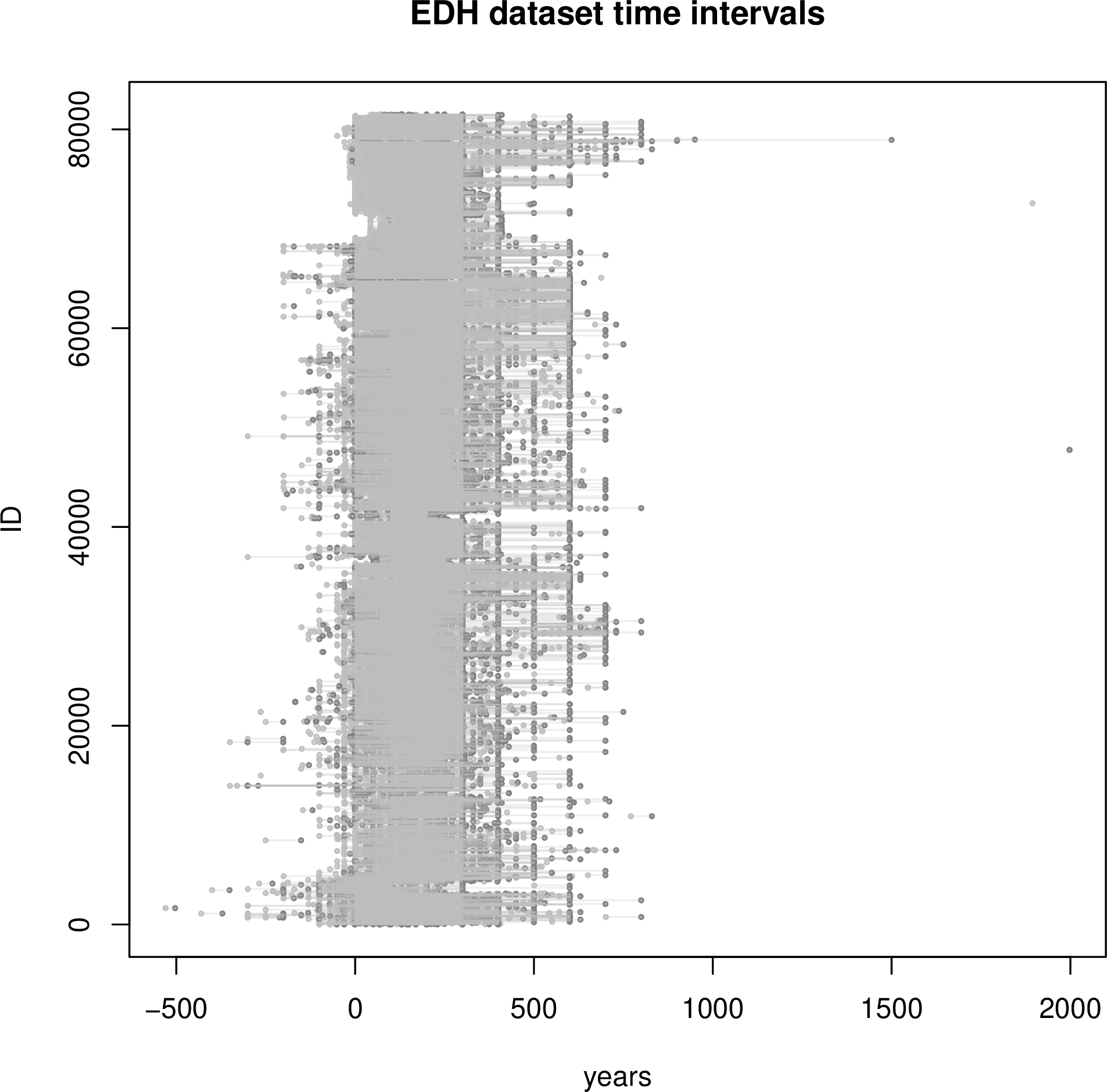
Plotting time intervals
To be able to plot efficiently time spans of existence of records in the EDH dataset, we
need to count with a numerical identifier.
# get IDs by removing alphabetic characters in id
R> ID <- as.numeric(sub("[[:alpha:]]+","",EDHdates$id))
A plot of relative dating for Roman inscriptions with ID is made with the [R] graphics
core package (or base package with R version 4.0.0).
# plot with graphics
R> plot(nb, ID, pch=20, col="#C0C0C0", xlab="Year", ylab="ID",
+       xlim=years, main="EDH dataset time intervals")
R> points(na, ID, pch=20, col="#808080")
R> segments(nb, ID, na, ID, col=grDevices::adjustcolor(8,alpha=.25))
or using the plot.dates() function from sdam
R> plot.dates(main="EDH dataset time intervals",
+             taq="not_before", tpq="not_after", cex=.5)
That produces:
Treating Outliers
By looking at the box-and-whisker plots below, we can clearly see a couple of outliers at least in each category.
# par(mfrow =  c(2, 1))
R> boxplot(nb, horizontal=TRUE, main="EDH 'not_before'")
R> boxplot(na, horizontal=TRUE, main="EDH 'not_after'")
That produces:
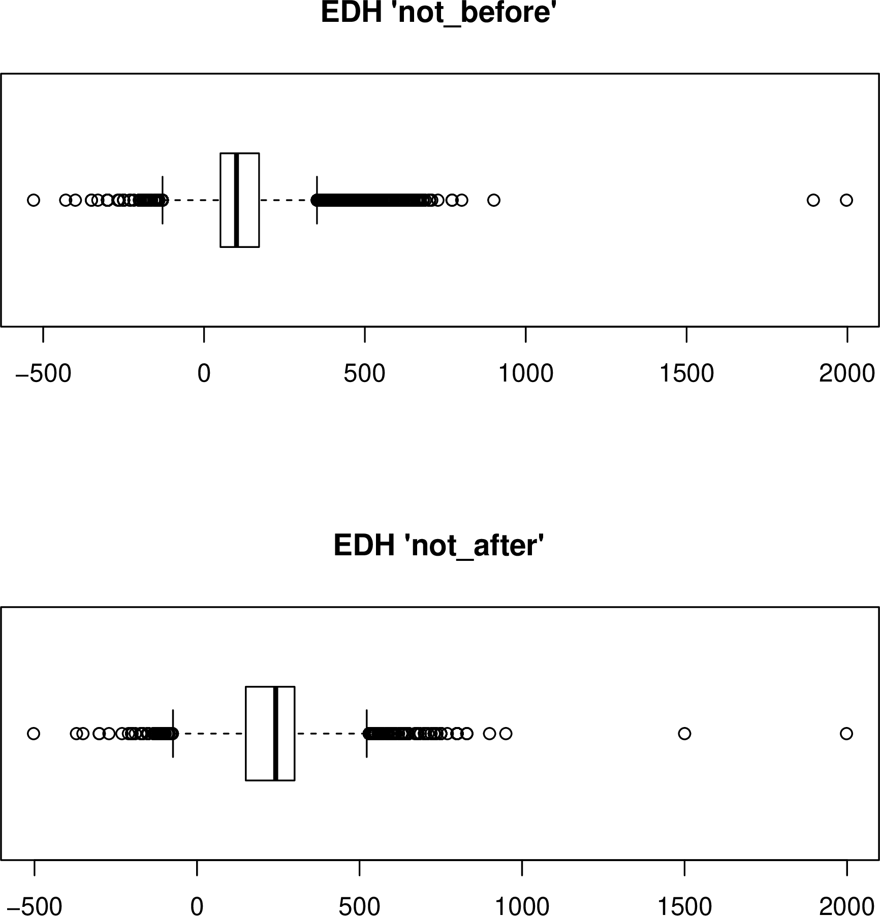
The two most extreme outliers in each category are given in $out produced by the boxplot() function.
# first outlier is the maximum value of the dates
R> outliers<- c(tail(sort(boxplot(nb, plot=FALSE)$out),2),
+               tail(sort(boxplot(na, plot=FALSE)$out),2))
#[1] 1894 1997 1500 1998
We remove these outliers in not_before and not_after, and we update the EDHdates object.
R> c(nb[which(nb %in% outliers)], na[which(na %in% outliers)])
#[1] 1997 1894 1998 1500

# update by removing outliers in both categories
R> EDHdates <- EDHdates[-c(which(nb %in% outliers),which(na %in% outliers)), ]
Since rows are removed from EDHdates, we need to update object identifiers to compute the
new the range of time.
# update values
R> ID <- as.numeric(sub("[[:alpha:]]+","",EDHdates$id))
R> nb <- as.numeric(as.vector(EDHdates$not_before))
R> na <- as.numeric(as.vector(EDHdates$not_after))

# new dates
R> years <- c(min(nb, na.rm=TRUE), max(na, na.rm=TRUE))
#[1] -530  950
Years are now between 530 BC and 950 AC. That is, from Archaic to Middle Byzantine chronological periods.
(See: Time and dating)
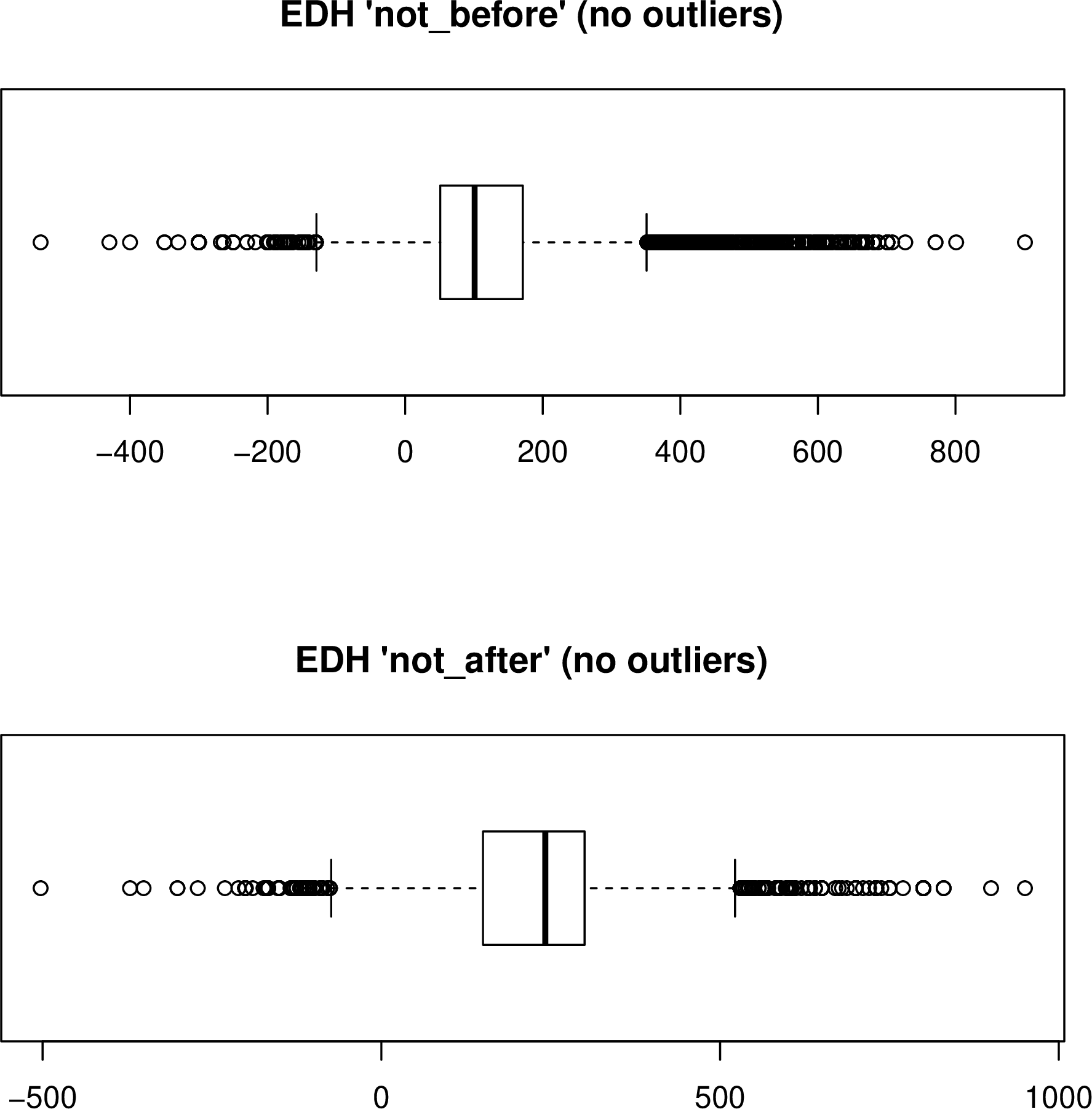
Plotting without outliers
Now we take a look at the box-and-whisker plots without outliers
# par(mfrow =  c(2, 1))
R> boxplot(nb, horizontal=TRUE, main="EDH 'not_before' (no outliers)")
R> boxplot(na, horizontal=TRUE, main="EDH 'not_after' (no outliers)")
that produces:
The next step is to plot relative dating without outliers and with updated range of time
and with plot.dates() function.
R> plot.dates(main="EDH dataset time intervals (no outliers)",
+       taq="not_before", tpq="not_after", out=2, cex=.5)
that produces a plot with no outliers:
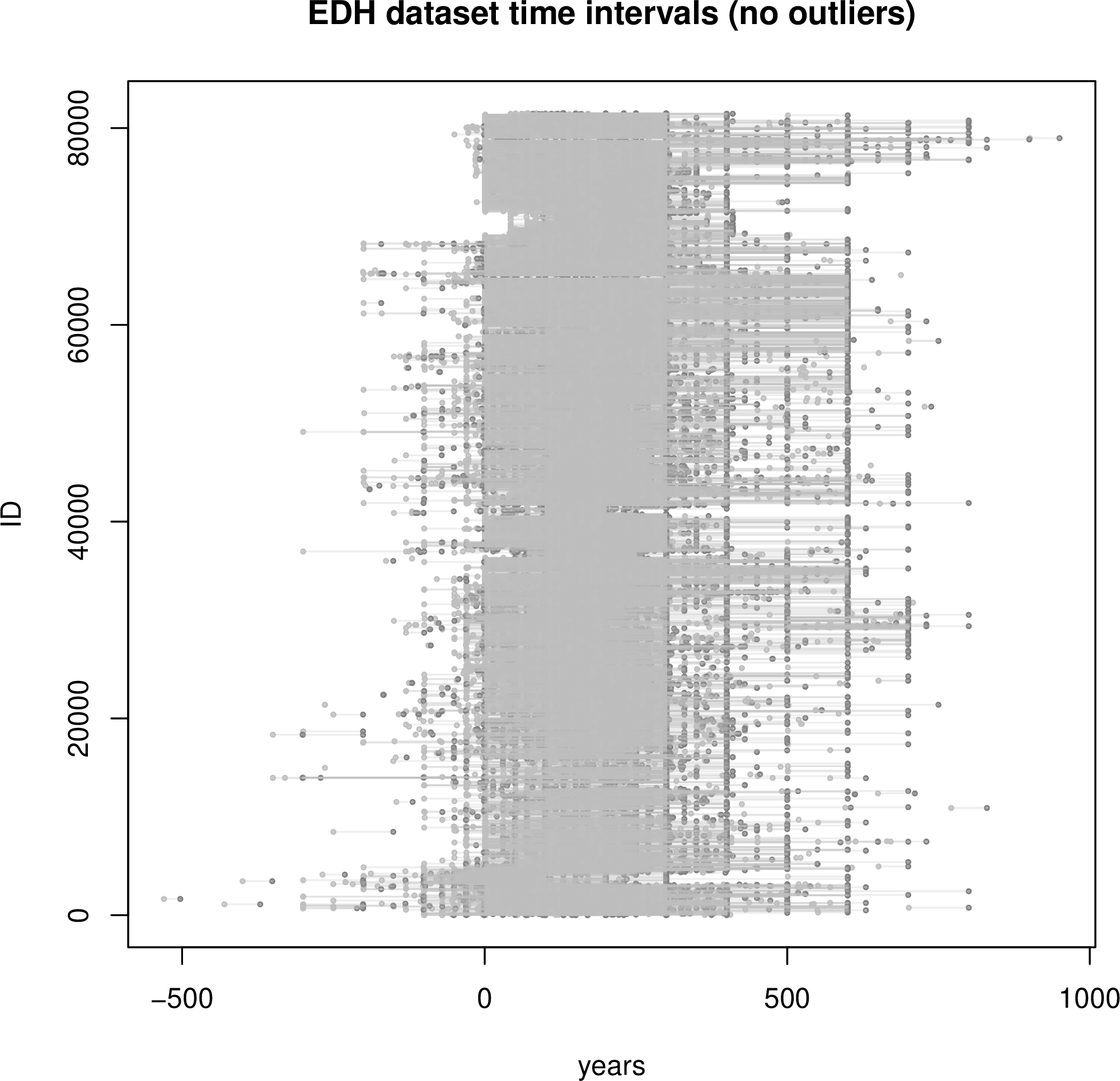
where we can see that most of the inscriptions in the EDH dataset are from
Early to Middle Roman.
Plotting time intervals
To plot time intervals, we use function plot.dates().
-
plot.dates()
Function usage
# use generic function
R> plot.dates(file=NULL, x=NULL, taq, tpq, out,
              main=NULL, xlab=NULL, ylab=NULL, xlim=NULL,
              pch, cex, col, lwd, lty, alpha, ... )
Parameters
Formal arguments of plot.dates() are:
x:
data frame object of variables and observations. If
NULLthenEDHdataset is takeny:
vector identifier (optional)
file:
path to file for a PDF format (optional)
taq:
TAQ or terminus ante quem
tpq:
TPQ or terminus post quem
out:
number of outliers to omit (integer or vector where first entry id for latest date)
Optional arguments from the graphics package for the plot are
main:
main tile
xlab:
xlabelylab:
ylabelxlim:
xlimit
And for the representation of time interval and boundaries of existence in the plot
pch:
symbol for taq and tpq
cex:
size of pch
col:
colors of pch and time interval segment
for time interval segments:
lwd:
width
lty:
shape
alpha:
alpha color transparency
…
additional parameters if needed