Epigraphic Networks using R
This post is about Epigraphic Networks based on measures of similarity of artefact assemblages and geographic proximity.
Measuring similarity of artefact assemblages and geographic proximity
To measure similarity of artefact assemblages and geographic proximity, [R] package
sdam provides the function simil(), which allows assesing similarity by comparing
columns representing –in this case– different attributes for epigraphic inscriptions.
Function usage
-
simil()
# arguments supported (currently)
R> simil(x, vars, type=c("sm","ja","ra"), uniq, diag.incl)
Which returns a square and valued matrix with similarity meassures based on simple match among variables.
Parameters
Formal arguments of simil() are:
x:
a data frame with an id column
vars:
(vector) column(s) in
xrepresenting attributes or variablestype:
whether the similarity measure is by simple matching
"sm", Jaccard"ja", or Rand index"ra"
Optional parameters
uniq:
(optional and logical) only unique elements?
diag.incl:
include entries in the matrix diagonal?
Note that at this point the ID column represents the labels of the nodes. In
case that an ID column does not exists, then the first column is taken
as id provided that there are not duplicated entry names in x.
Similarity measures
For cases where duplication does not matter, a good option is Jaccard similarity whose index is the proportion of the number of observations in both sets to the number in either set. This index is formally expressed as \(J(A,B)= \left| A \cap B \right| / \left| A \cup B \right|\). (Otherwise
Todo
Rand index plain and corrected by chance.
Structures of similarity in the EDH dataset
We illustrate the use of the simil() function with ancient inscriptions from
the Epigraphic Database Heidelberg, and we first follow the entry Epigraphic Database Heidelberg
to see how accessing the EDH dataset using sdam [R] package.
# devtools::install_github("mplex/cedhar", subdir="pkg/sdam")
# devtools::install_github("sdam-au/sdam")
R> library("sdam")

# load the EDH data from this package
R> data("EDH")
Epigraphic network data
Creating epigraphic network data list with variables measures of similarity of artefact assemblages and geographic proximity.
For example, a list object named epinet with the ID of the inscription plus seven other characteristics from
the EDH dataset is produced by edhw().
# choose variables of interest and record it as a data frame
R> epinet <- edhw(vars=c("type_of_inscription", "language", "material", "country",
                  "findspot_ancient", "not_after", "not_before"), as="df")
Take a look at this data:
# first eight entries in the data frame
R> head(epinet, 8)
#        id   type_of_inscription not_before not_after                                material language findspot_ancient country
#1 HD000001               epitaph       0071      0130                Marmor, geädert / farbig    Latin       Cumae, bei   Italy
#2 HD000002               epitaph       0051      0200       marble: rocks - metamorphic rocks    Latin             Roma   Italy
#3 HD000003 honorific inscription       0131      0170       marble: rocks - metamorphic rocks    Latin             <NA>   Spain
#4 HD000004    votive inscription       0151      0200    limestone: rocks - clastic sediments    Latin    Ipolcobulcula   Spain
#5 HD000005               epitaph       0001      0200                                    <NA>    Latin             Roma   Italy
#6 HD000006               epitaph       0071      0150    limestone: rocks - clastic sediments    Latin      Sabora, bei   Spain
#7 HD000007               epitaph      -0100     -0051 travertine: rocks - chemische Sedimente    Latin             Roma   Italy
#8 HD000008               epitaph       0101      0200       marble: rocks - metamorphic rocks    Latin            Roma?   Italy
For instance, entry 8 indicates that this ancient findspot is uncertain.
Function cln()
R> epinet2 <- cln(epinet)
And then we take a look at epinet2 again, and we assume the questioned entries.
# first eight entries in the new data frame
R> head(epinet2, 8)
#        id   type_of_inscription not_before not_after                                material language findspot_ancient country
#1 HD000001               epitaph       0071      0130                Marmor, geädert / farbig    Latin       Cumae, bei   Italy
#2 HD000002               epitaph       0051      0200       marble: rocks - metamorphic rocks    Latin             Roma   Italy
#3 HD000003 honorific inscription       0131      0170       marble: rocks - metamorphic rocks    Latin               NA   Spain
#4 HD000004    votive inscription       0151      0200    limestone: rocks - clastic sediments    Latin    Ipolcobulcula   Spain
#5 HD000005               epitaph       0001      0200                                      NA    Latin             Roma   Italy
#6 HD000006               epitaph       0071      0150    limestone: rocks - clastic sediments    Latin      Sabora, bei   Spain
#7 HD000007               epitaph      -0100     -0051 travertine: rocks - chemische Sedimente    Latin             Roma   Italy
#8 HD000008               epitaph       0101      0200       marble: rocks - metamorphic rocks    Latin             Roma   Italy
The countries in epinet2 are:
# need first to unlist the component object
R> unique(unlist(epinet2$country))
# [1] "Italy"                  "Spain"                  "United Kingdom"         "Portugal"
# [5] "France"                 "Libyan Arab Jamahiriya" "Germany"                "Hungary"
# [9] "Austria"                "Bulgaria"               "Bosnia and Herzegovina" "Montenegro"
#[13] "Netherlands"            "Tunisia"                "Romania"                "Algeria"
#[17] "Jordan"                 NA                       "Croatia"                "Switzerland"
#[21] "Belgium"                "Albania"                "Serbia"                 "Egypt"
#[25] "Syrian Arab Republic"   "Morocco"                "Turkey"                 "Lebanon"
#[29] "Kosovo"                 "Macedonia"              "Slovakia"               "Greece"
#[33] "Slovenia"               "Iraq"                   "Israel"                 "unknown"
#[37] "Vatican City State"     "Ukraine"                "Cyprus"                 "Yemen"
#[41] "Sudan"                  "Luxembourg"             "Czech Republic"         "Malta"
#[45] "Poland"                 "Armenia"                "Monaco"                 "Azerbaijan"
#[49] "Sweden"                 "Denmark"                "Moldova"                "Saudi Arabia"
#[53] "Uzbekistan"             "Liechtenstein"          "Georgia"
Subsetting the data
For example, we use the base [R] function subset() to substract epigraphic material in “Greek-Latin” from Egypt.
# a subset of a subset
R> subset(subset(epinet2, country=="Egypt"), language=="Greek-Latin")
#            id        type_of_inscription not_before not_after    material    language findspot_ancient country
#2003  HD002003 identification inscription      -0116        NA          NA Greek-Latin           Philae   Egypt
#23091 HD023091                         NA       0145        NA Holz, Wachs Greek-Latin               NA   Egypt
#23138 HD023138         votive inscription      -0029        NA          NA Greek-Latin            Syene   Egypt
#27345 HD023091                         NA       0145        NA Holz, Wachs Greek-Latin               NA   Egypt
#27351 HD023138         votive inscription      -0029        NA          NA Greek-Latin            Syene   Egypt
#32500 HD030147                         NA       0010      0011          NA Greek-Latin       Alexandria   Egypt
#34436 HD032079                         NA         NA        NA          NA Greek-Latin          Schedia   Egypt
#51198 HD048625 identification inscription       0006        NA          NA Greek-Latin         Berenice   Egypt
#54194 HD051485                         NA       0155      0225          NA Greek-Latin       Alexandria   Egypt
#58318 HD055974                         NA       0001      0200          NA Greek-Latin         Berenice   Egypt
#70110 HD067781   public legal inscription      -0037     -0030          NA Greek-Latin      Leontopolis   Egypt
Ranked frequency
A ranked frequency of different kinds of inscriptions including missing information is computed as follows:
R> as.data.frame(sort(table(unlist(epinet2$type_of_inscription), useNA="ifany"), decreasing=TRUE))
#                              Var1  Freq
#1                          epitaph 28522
#2                             <NA> 22222
#3               votive inscription 14683
#4         owner/artist inscription  5164
#5            honorific inscription  4338
#6  building/dedicatory inscription  3450
#7                mile-/leaguestone  1766
#8       identification inscription  1600
#9                      acclamation   525
#10                military diploma   507
#11                            list   363
#12                         defixio   311
#13                           label   287
#14            boundary inscription   258
#15        public legal inscription   256
#16                         elogium   154
#17                seat inscription    88
#18                          letter    81
#19                          prayer    57
#20       private legal inscription    37
#21         assignation inscription    15
#22                        calendar    14
#23                     adnuntiatio     3
That is, a decreasing sorted table given as data frame of the type_of_inscription
component of epinet2. Since epinet2 is a list object, it is required to “unlist” the
data object to produce a table with the frequencies.
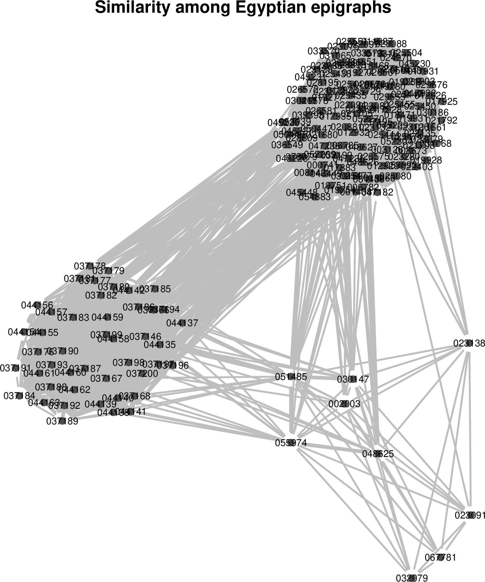
Example: Similarity among Egyptian epigraphs
We can compute similarity among Egyptian epigraphs with function simil().
For this, we look at the attribute types stored in different columns.
R> as.data.frame(colnames(epinet2))
#    colnames(epinet2)
#1                  id
#2 type_of_inscription
#3          not_before
#4           not_after
#5            material
#6            language
#7    findspot_ancient
#8             country
For instance, in case we want to choose "type_of_inscription", "material", and "findspot_ancient",
these correspond to columns 8, 5, and 3.
Similarities among Egyptian epigraphs by simple matching or default type "sm" with the above attribute variables are recorded in
a matrix object named epEgs where the ID in epinet2 corresponds to the dimensions labels.
# similarity function on the subset for the three variables
R> epEgs <- simil(subset(epinet2, country=="Egypt"), vars=c(8,5,6))

# number of rows in this square matrix
R> nrow(epEgs)
#[1] 170
And then we look at some cell entries
# similarity between the first six inscriptions in 'epEgs'
R> epEgs[1:6, 1:6]
#         HD000744 HD002009 HD003137 HD006817 HD006820 HD008184
#HD000744        0        1        1        0        0        0
#HD002009        1        0        0        0        0        0
#HD003137        1        0        0        0        0        0
#HD006817        0        0        0        0        1        0
#HD006820        0        0        0        1        0        0
#HD008184        0        0        0        0        0        0
where we observe six records of a single similarity.
Plot similarities
To produce a graph for the similarity among Egyptian epigraphs, we employ the [R] package multigraph that
depends on multiplex.
# define scope for the graph
R> scp <- list(directed=FALSE, valued=TRUE, ecol=8, pos=0)

# load "multigraph" where "multiplex" gets invoked
R> library(multigraph)

# plot similarity graph of 'epEgs' for the chosen variables
R> multigraph(epEgs, scope=scp, layout="force", maxiter=70, main="Similarity among Egyptian epigraphs")